Radius of Curvature
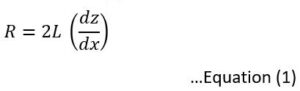
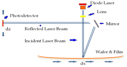
From measured data, the radius of curvature is calculated using Equation (1). Here,
R = Radius of curvature
L = Beam path distance from wafer surface to the detector
dx = horizontal displacement of the laser
dz = vertical displacement of the detector
Example:
A 20M diameter calibrated curved mirror is used. While scanning, for every 1-mm of laser beam travel (dx), the detector position is measured to be changing 30um. The beam path of the system is 333 mm (typical)
R = 2x333x (30um)/(1mm)
= 666x30x10-6/1×10-3
= 20
Bow Height
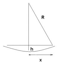
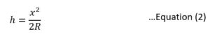
Bow height can be calculated with respect to the diameter and radius of curvature using this equation:
Assumptions
- a) Spherical surface only
- b) Bow height, h << x (scan path) << R (radius of curvature)
For a Spherical Surface
(R-h)2 + x2 = R2
Or, R2– 2Rh+ h2 + x2 = R2
Or, h = x2 / 2R (ignoring the h2)
Bow Height , h = x2 /2R
h= Bow height
x= Radius of the sample wafer
Example
A calibrated mirror with 50 mm physical radius and 20M curvature radius is used.
Now, the bow height = x2 / 2R = (50×10-3 )2 / 2(20) = 2500×10-6/40 = 62.5um
Stoney’s Equation (using Radius of Curvature)
Stoney’s equation (3) is used as a stress–radius relationship of a stressed wafer:-
Where,
E = Young’s Modulus
Ts = Substrate Thickness
Tf = Film Thickness
v = Poisson’s Ratio
R = Change is the radius of curvature before and after film
Here,  is defined as the stress constant. For Silicon, 180.5 GPa is used.
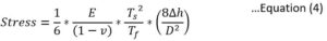
Stoney’s Equation (using Bow Height)
Combing equation 2 and 3
Steps for the Tool:
1. 1st-Map: First Map->[#line=4, Laser Freq=780, Film thickness=0, Wafer thickness=0.5, Wafer size=200, Scan Size=180)->Run.
2. StressConstant: Setup->System->Preset->Put (Stress Constant value in Pa*10)->Ok
3. Recipe: Setup->Recipe (Check values)->Save-> (give name)->OK
4. 2nd Map:
(a ) File->Open->(1st Map file)
(b) Setup->Recipe->Load (target recipe)->OK
(c) 2nd Map-> (Check values, film thickness is 1um=10000 A)-> Run
5. Compare: Make sure the tool and excel get correct values (use the red vaues as reference).
Now expect both excel and tool values to closely match.
Example:
| (A) Get pre and post measurement values from FSM128 | Excel Input | Tool Input |
| Measured 1st Radius =R1 (M) | 84.017 | |
| Measured 2nd Radius =R2 (M) | 62.523 | |
| Measured 1st Bow =h1 (um) | 59.512 | |
| Measured 2nd Bow =h2 (um) | 79.971 | |
| (B) Known values | ||
| Es=63GPa (Young’s Modulus) | 63000000000 | |
| Vs=0.2 (Poisson’s Ratio) | 0.2 | |
| Ts=0.5mm (Wafer thickness) | 0.0005 | 0.5 |
| Tf=20um (film thickness, 1um=10,000A) | 0.00002 | 200000 |
| D=200mm (wafer diameter) | 0.2 | 200 |
| (C) Calculate Stress uisng Eq 3 or 4 | ||
| Term1=Const (1/6) | 0.166666667 | |
| Term2=Stress_Constant= Es/(1-Vs) | 78750000000 | 787500000000 |
| Term3= Ts^2/Tf | 0.0125 | |
| Term4A=(1/R2-1/R1) … using radius (Eq. 3) | 0.004091761 | |
| Term4B= (8*(Bow2-Bow1)/D2)…using bow (Eq. 4) | 4091.8 | |
| Outputs | Excel Output | Tool Output |
| Stress_Radius(MPa)=(Term1*Term2*Term3*Term4A)/1000000 | 0.671304551 | 0.671404551 |
| Stress_Bow(MPa)=(Term1*Term2*Term3*Term4B)/1000000 | 0.671310938 | 0.671440938 |
01. What is heat recipe?
A recipe file which controls temperature increment time, steps and rate.
02. How can we create one heat recipe file?
We need a machine that supports wafer measurements with heat (500TC, 900TC etc). From the right sidebar (Fig 1) we need to press Heat button. A new window will appear (Fig 2). We have to set values according to our experiments in the white box. Then press Run.
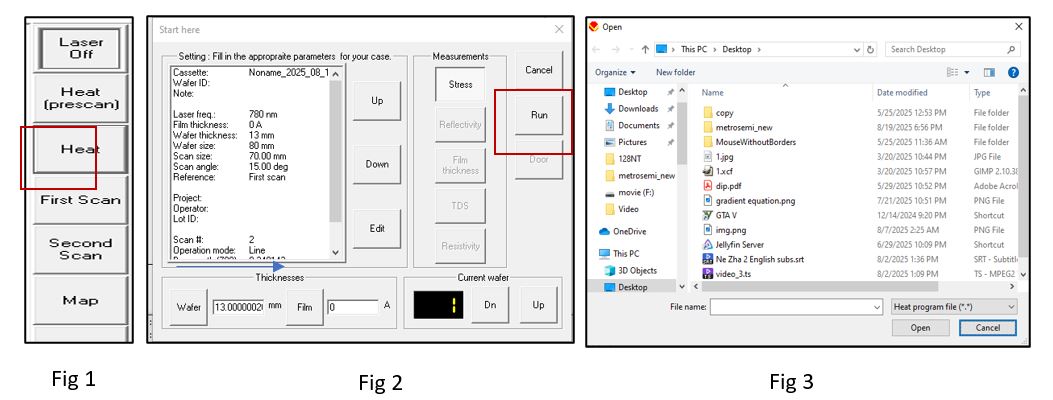
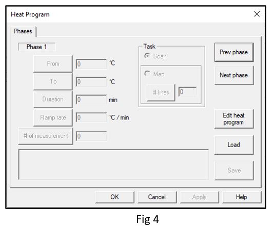
When Run is pressed the software will ask us to select a heat recipe file. As we don’t have any file present will select cancel in fig 3. Then we will have a window (Fig 4) in where we will create our heat recipe. We need to select the button Edit heat program. Which will enable us to input values to the text boxes. If we want to start at 50C temperature and finish at 4000C then we need to fill From and To text boxes. We need to fill either Duration or Ramp rate. If we fill one box, the software will auto fill the other box for us. Finally, we need to fill the box with #of measurements. Then the software will select the temperature points where to measure the wafers.
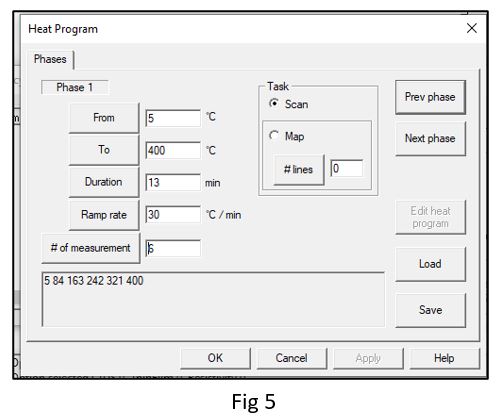
After adding all the information, the window should look something like this (Fig 5). If we want to add more phases then we can select next phase and continue the process. If we are done then we can press Save and save our heat recipe in our desired location. If we don’t want to save the heat recipe, we can directly use it by pressing OK.
03. How can we load heat recipe file?
For load a recipe file we need to select Heat from Fig 1. Then after given the necessary parameters in the window (Fig 2) press Run. Then fig 3 window will appear. We need to browse to our recipe file and open it. Then we can see it loaded in a window like fig 5. We now can press Ok to use the file.
04. How can we update heat recipe file?
We can update it in two different ways. First, we can open it in our software. The we can edit the values in the window (Fig 5). We can press Ok to use it or Save to save the file with updated value.
Another approach is to open the file directly using notepad. We can right click it and open with notepad.
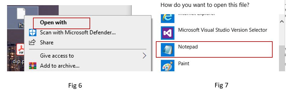
The file would look like fig 6. First value is number of phases. Here it’s 2. Each next line
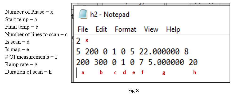
Represents a Phase. For each line, the first value is the stating temperature, second value is the ending temperature. Third value is number of lines to scan. If fourth value is 1, then it’s a scan. If fifth value is one then it’s a map. Next value is number of measurements. Last two value is ramp rate and duration of scan. We can change the values in the file and save it to change the recipe.